I haven't published in a while since I got a job making websites. I suppose writing and coding partly lost their escapist factor, being able to make a living out of it. But this week, I visited a hackerspace and it inspired me to log my creativity again.
A hackerspace is where people play with technology the way it should be. There's something amazing about hobbyist passion, free from life's obligations. According to their site,The hacker culture is a subculture of individuals who enjoy the intellectual challenge of creatively overcoming the limitations of current technologies to achieve novel and clever outcomes. I enjoyed the extremely nerdy vibes, and I mean that in the best way. We played pong and snake on a handmade table with a 32*32 LED light grid built into it, hooked up to NES controllers. They have a microscope, 3D printer, woodturning kit, self-checkout bar, and lots of hacky projects, all of which are somewhat work in progress. They got enthousiastic about AI technology and the demoscene. And it's an open non-profit without entry fees. Anyhow, seeing the low-res LED grid table made me wonder if I could run the evomatrix life simulation on it. And so I revisited the project and noticed some problems.

Python performance struggles
The main thing I wanted to fix was the speed. It was quite unoptimized. I started with the graphics. I used Python 2.7 with TKinter in the first version of evomatrix. This time I used python3 and pygame for the visuals. The graphics code runs a lot faster now, but admittedly, I simplified it and the surface only use as many pixels as there are cells.
To keep track of performance, I used the time.perf_counter to clock time passed at different points of execution. The results were unexpected. I thought I would lose a lot of time with updating values in the 2D-arrays, but that was not the case at all. The performance gains from improving the random generation were also minimaL. Lookups of values, and if-statements, were more costly. And my biggest surprise, using numpy for all the 2D-arrays (or matrixes, as they are called in numpy) slowed the simulation considerably, instead of making things run faster.
Numpy has great functions to help with matrix calculations, and since the simulation uses 5 matrixes which are checked and updated constantly, I thought I could make some serious gains here. But what numpy is good with are calculations on big chunks of data in those matrixes. Multiplying entire matrixes, transforming them and so forth. What I am doing instead is checking every cell one by one. And iterating over a numpy matrix is actually slower than iterating over a default python matrix. Rewriting the code to make all the operations on a larger scale was no use because the costly operations like moving have to be handled on a cell-by-cell basis. I also thought I could save computing time by storing every value as an 8-bit unsigned integer (dtype=uint8). But for regular calculations, this special numpy data type is implicitly converted to a data type python can do regular operations on. This inefficiency can largely be relieved by making the conversion explicit, for example int(grid[x,y]). But in the end, all this unpacking and repacking was only making matters worse. I ditched numpy again and ended up not far from where I started. I suppose that if I really want a fast-running simulation, I should try a more low-level language. For now, I get 100 FPS on a 32x32 grid, which means around 100.000 cells are updated and redrawn every second, and that's fine.
Better speciation
Some other changes I made were more succesful, and made the evolution more logical and interesting. For example, one big issue with he previous version was that individuals would live forever, staying in their cells if they don't move, and evolution would stagnate. I then had to introduce disruption, random deaths, to solve this. In the new version, if individuals have enough energy to reproduce but no free space to put their offspring, they will produce offspring on top of another cell, replacing it. This way, generations are replaced at a regular pace and faster growing organisms can still outcompete slower growing organisms without direct fighting.
Basic rules of the simulation: Cells have 3 genes, represented by red, green and blue light (search for 'rgb colorspace' if this is not intuitive). The first cell is mostly green, allowing it to get energy by doing nothing at all. Cells without any green mixed into them can instead gain energy when they win a fight with another cell. The blue gene makes a cell move around more. This allows it to spread faster, but also costs energy. And if it moves onto another cell, they fight. The red gene determines how much damage is inflicted a fight, as a percentage of energy taken away from the other cell. To make use of that energy, the cell needs to be not-green. Having red genes also costs energy. Cells reproduce asexually when they are at around 80% of their maximum energy level and pass some of their energy to their babies. These babies differ slightly from their parents.
One result of this is that after an initial period of allopatric speciation followed by a plethora of short-lived atypical species, there is now a clear rock-paper-scissor mechanic with 3 stable species. There are plants (bright green) which sit still and grow fast, overgrowing other plants. There are herbivores (orange to purple), who move and eat the green plants, burning through them like a fire. And then there are yellow plants, which can defend themselves against the herbivores but which get overgrown by green plants.
There are two more varations. I don't dare call them seperate species, even though they take up a different niche and have different genes, because they die off and re-evolve on ecological (not evolutionary) timescales. So phylogenetically, they are just temporary variations of other species. They include plants in open spaces, which evolve teal hues (more blue = faster) to colonize the available open space. And then there are the more brightly colored herbivores, who can eat plants extremely fast and win fights, but only survive as long as they are in the middle of a forest. Once the forest is eaten, they wither away quickly and the slightly duller, less aggressive but more long-lived herbivores carry on the herbivore genes. In the 3 species stable system, species are highly specialized but there is still variation in color. I don't know the main reason, though 3 effects probably play a role: either selection pressure just isn't strong enough to counter genetic drift, another possibility is that populations go through bottlenecks so often that there is a significant founder effect, and finally it could be that the variation is an actual reflection of a changing environment. In smaller resolutions, herbivores sometimes go extinct, but they always re-evolve in the belly of the resulting forest. It's interesting that when herbivores go extinct, yellow and teal plants go extinct as well. This makes sense, because in a dense forest of only plants there is no more benefit for trying to move to an open space or for defending against herbivores.
Four species system
The existence of teal, actively moving plants made me wonder if a fourth species could be stable by tweaking the configuration. And sure enough, by making movement very cheap, it is possible to get an equilibrium with 4 species. For this I also made the simulation a bit larger, and made the rate of mutation decrease gradually. With that last change, evolution doesn't keep creating new variations by drift or local conditions, but 'zooms in' on the species that can survive long-term. After enough time without mutation, there are no longer any differences between individuals of the same niche.
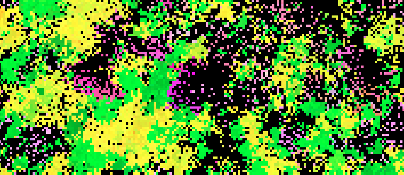
At the start, mutation is high and many species radiate in what looks like fireworks::
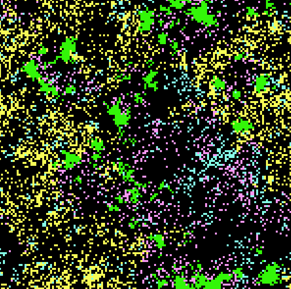
But after mutation is taken away and a long time has passed, only four survive:
The final system is a little bit more difficult to understand. The interaction of non-moving, non-combative, fast growing plants with frantic herbivores is straightforward. But then there are two more species, teal and yellow, which are both diffuse and tend to swarm around the same areas, but need the green-purple system to stay stable. The yellow species, unlike in the previous simulation, now moves as well. It is about 30% as mobile as purple or teal are, which is enough to spread out. It is still entirely autothrophic, so it doesn't gain energy from catching other cells in this movement. The movement helps its survival chances in 2 ways. It spreads out to new areas without predation, and secondly it creates a sort of maze or breakwater that wears out waves of purple and teal. Teal is not actually dangerous as a predator, but grows almost as fast as green while moving, so it could easily overgrow yellow otherwise. Teal is the most vulnerable species. It grows a little bit slower than green and loses any fight with yellow or purple it gets into. It provides a great snack for purple, which dies after not feeding for only a short while. But thanks to teal, even the open areas provide snacks to weary travelers every few pixels. Teal's strategy is to keep moving and growing, to be the first to colonize new areas and to survive in small numbers between the other species. In a way, purple, the only species in a higher trophic level (eating other species) is a keystone species. Without it, green would overgrow everything and diversity would be minimal. It's crazy that 3 one-dimensional genes can lead to 4 entirely different species. The earlier, non-moving yellow species and the darker shades of purple did not survive as they are outcompeted by their paler cousins in the long term.
 You get used to it. I… I don't even see the pixels. All I see is forest, herbivore, cactus.
This possibly shows the maximum ecological diversity with these 3 single-purpose genes, but it's hard to tell for sure.
With some luck, I can find a way to run the simulation on the LED coffee table at the hackerspace.